Changelog

• 0.3

  Mar 19, 2025

  Dhanush Kovi

  Streamlining Training Process

  The major rewrite is now complete 🎉!

  The training process has been simplified and can now be run easily.

  

  🔄 Training the model

  A YAML configuration file is used for training parameters. For example, the following configuration is used for 2D Burger’s Equation:

  device: "cuda"
  learning_rate: 0.01
  Nb: 1000
  Nf: 5000
  
  model:
    input_dim: 3
    hidden_layers: 4
    hidden_units: 20
    output_dim: 2
    epochs: 6000

  You can train an example model using the following parameters by:

  uv run main.py [--model pinn|pikan] [--config <config_path>] EXAMPLE

  The default value of type and config are set to pinn and <default_example_path> respectively. For example, to run burger2d using PIKAN model:

  uv run main.py --model pikan burger2d

  🛠️ Refactored Examples

  The examples are now simplified in the generation of input points. Instead of using multiple functions with similar parameters between them, a single generate_data() function is used.

  ✨ New Progress Indicator

  The training progress is now shown via progress bar in terminal using the alive-progress library.

  Epoch 30, Loss: 0.120250269771 |████████████████████████████████████████| 30/30 [100%] in 4.6s (4.53/s)

  You can find our repository under gulfgap/gulfgap!

• 0.2

  Mar 7, 2025

  Dhanush Kovi

  Sneak Peek into Modular Rewrite

  

  We have an early update this time! After stabilizing the 2D Equations, we’ve started a major rewrite converting all Jupyter notebooks to Python modules across the project.

  Regression fix in calculation of gradients

  During the sprint, we’ve identified a regression during the calculation of gradients in the loss function. The gradients are calculated multiple times using torch.autograd.grad aganist each input variable, rather than input tensor. While this might seem more intuitive, the difference in memory usage is enormous.

  There’s a slight uptick in the loss (on the order of 1e-10) after the fix, but the overall memory usage has dropped significantly with large amounts of data, making the benefits far outweigh the cons.

  Improved dependency management

  Using uv for package and dependency management allowed us to install dependencies and test the code in isolation faster. You can find more about uv on their blog.

  Stay Tuned for more!

  Although this changelog is small, we have much more to say! You can also find our repository at the footer of this website.

  • At the time of writing, the repository is inaccessible. We plan to make it public soon!
• 0.1

  Mar 4, 2025

  Dhanush Kovi

  Stabilizing 2D Equations for Physics Informed Networks

  

  Previously on GulfGap, we’ve finished working on 2D Burger’s Equation (which will be released later) during which we’ve started observing instabilities in 2D Equations. In the case of 2D Burger, the network was stabilized by adding a layer before output that enforces boundary conditions using a linear interpolation equation. This layer is called Boundary Encoding Layer.

  Sadly, this layer requires careful tweaking of initial conditions and boundary conditions. Altering the conditions for all equations is not ideal for a long-term solution.

  After looking through various sources, we’ve solved this by a straightforward solution.

  • Rather than returning all output variables through a single layer at the end, each variable now has its own layer.

  Why did this work?

  In many physics applications, different outputs often represent different physical quantities (for example, velocity vs pressure) that may have different scales, boundary conditions or error sensitivites. When layers are separated into their own weights and biases, the network can tailor the learning dynamics for each quantity.

  In contrast, a single layer with multiple targets forces all outputs to share the same weight matrix, making it less optimal for such applications.

  Observations for other equations

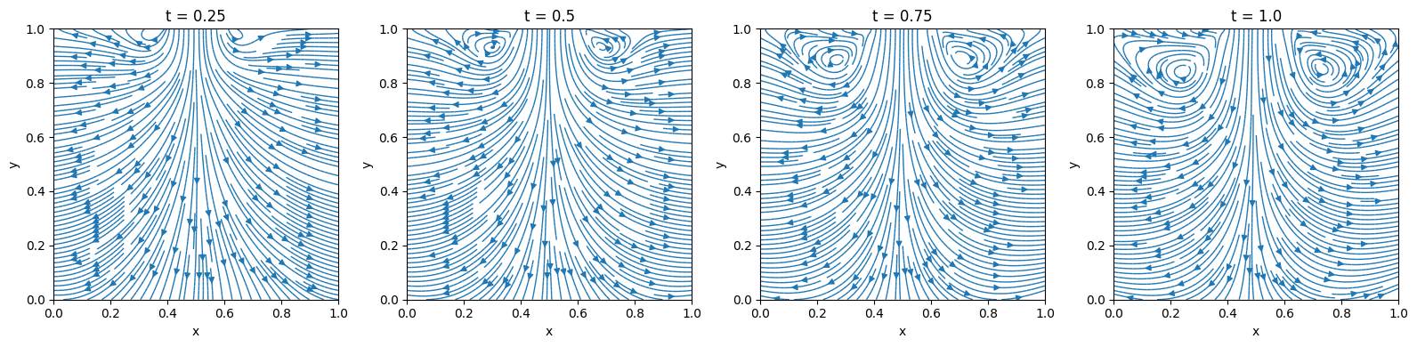
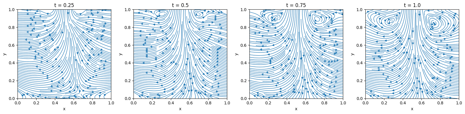
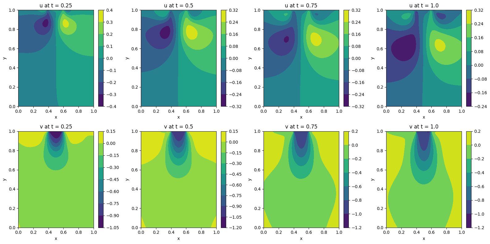
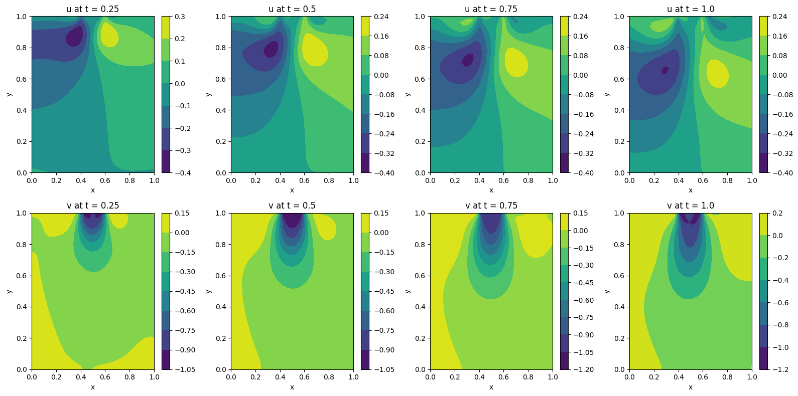
  Based on the prior changes, the following observations were obtained for unsteady flow equations of: Lid-Driven Square Cavity and Channel Flow with Jet Impingement Problems.

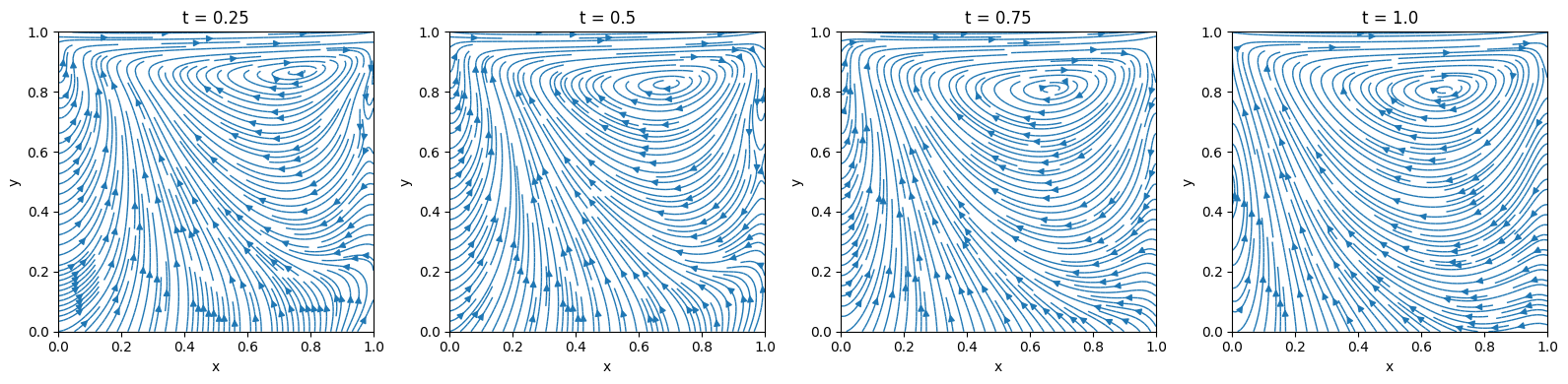
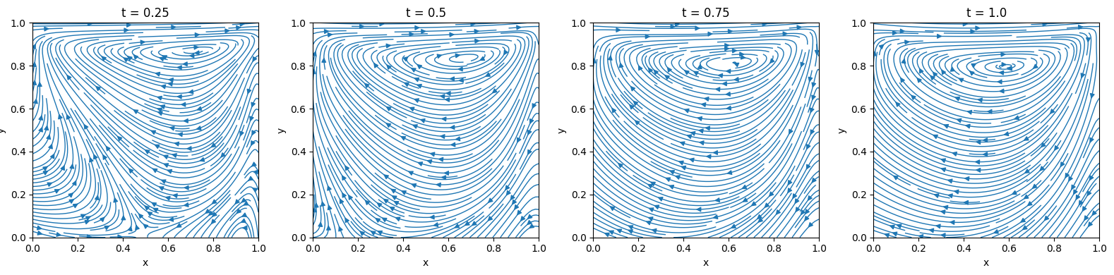
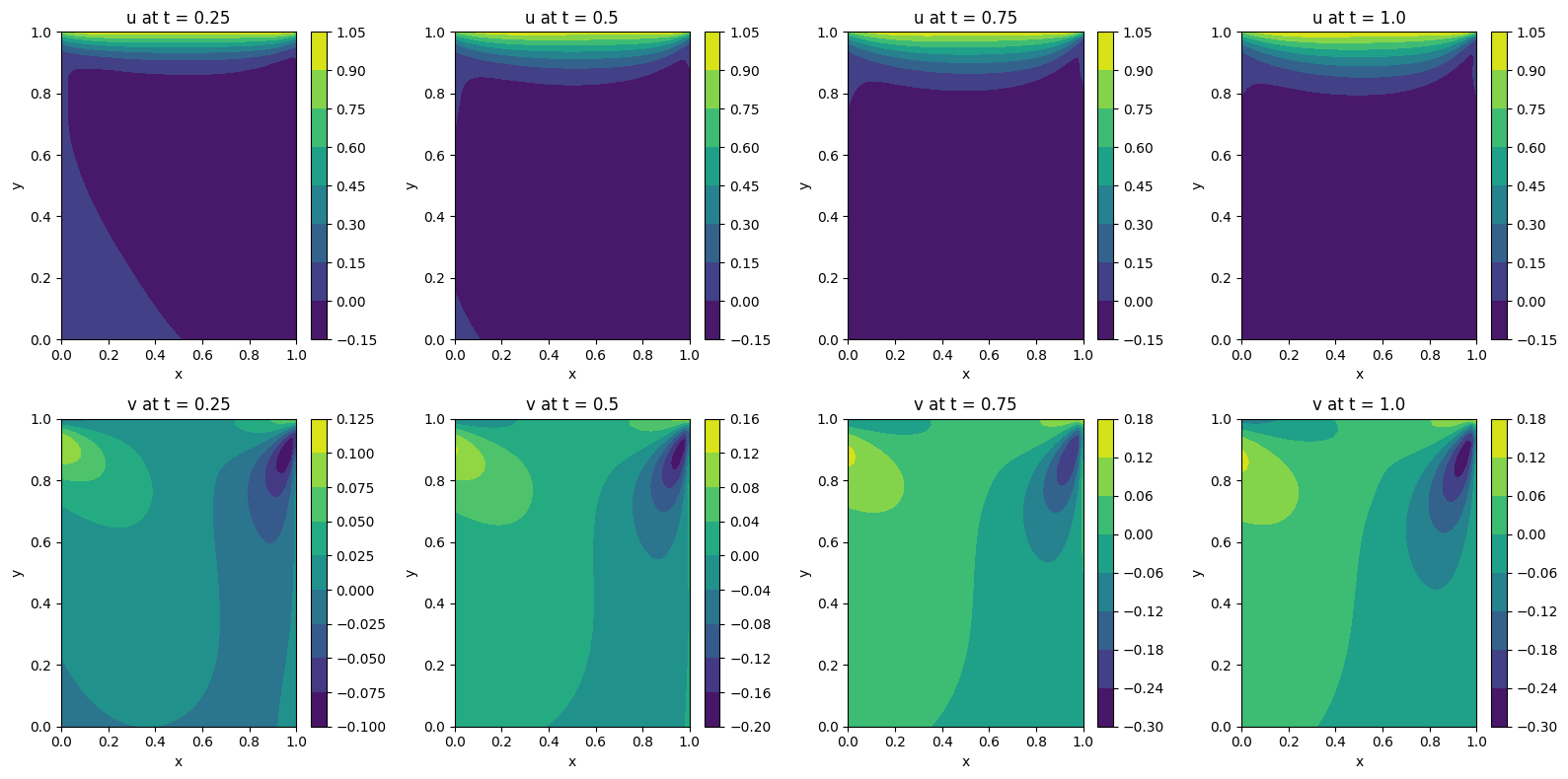
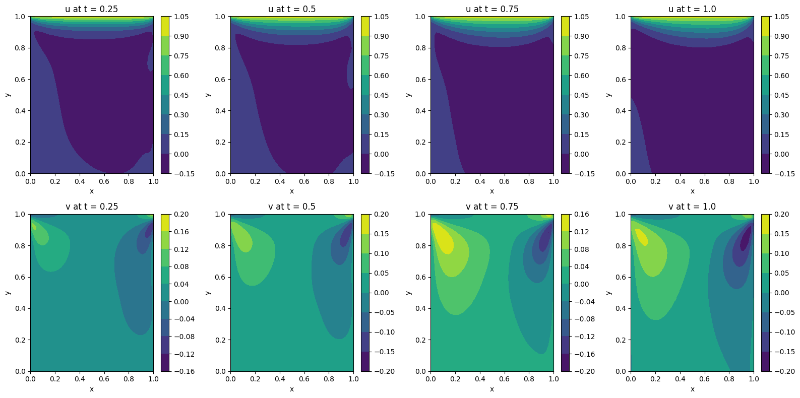
  Lid-Driven Square Cavity

  

  

  Similarly, the contours of both velocity components (along horizontal and vertical directions) can be plotted at various time intervals for observing changes of each velocity component over time.

  

  

  Channel Flow with Jet Impingement

  

  

  Similarly, the contours of both velocity components (along horizontal and vertical directions) can be plotted at various time intervals for observing changes of each velocity component over time.

  

  

  • Pressure Poisson Equation can be removed from loss calculation. There are two reasons for this decision.
    • Pressure Poisson Equation is derived from other two equations (continuity and momentum equations).
    • Pressure constraints throughout the network can be enforced in a non-rigid manner.
  • The network’s sensitivity to initial conditions has reduced in this method.
  • The absence of hard enforcement of BCs in solving other equations suggests that Boundary Encoding Layer is superfluous in the case of 2D Burger’s Equation.

  …was the Boundary Encoding Layer even needed in the first place?